Vendor-neutral sequences and their implications for the reproducibility of quantitative MRI
This living preprint encapsulates the code, data and runtime (R and Python) for an interative exploration of our findings from Karakuzu et al., 2022.
1🎬 Introduction
1.1What is VENUS?
VENUS is the acronym of our vendor-neutral qMRLab workflow that begins with the acquisition of qMRI data using open-source & vendor-neutral pulse sequences and follows with the post-processing using data-driven and container-mediated qMRFLow pipelines (Figure 1).

Figure 1:Schematic illustration of the VENUS components.
Open-source and vendor-neutral pulse sequences are developed as RTHawk applications, that can be run on most GE and Siemens clinical scanners.
1.2NATIVE vs VENUS: Does it matter to the measurement stability?
The purpose of this study was to test whether VENUS can improve inter-vendor reproducibility of T1, MTR and MTSat measurements across three scanners by two vendors, in phantoms and in-vivo.
To test this, we developed a vendor-neutral 3D-SPGR sequence, then compared measurement stability between scanners using VENUS and vendor-native (NATIVE) implementations.
Toggle the tabs for details:
- G1 GE Discovery 750w (3T)
- S1 Siemens Prisma (3T)
- S2 Siemens Skyra (3T)
- G1 SPGR (
DV25.0_R02_1549.b) - S1 FLASH (
N4_VE11C_LATEST_20160120) - S2 FLASH (
N4_VE11C_LATEST_20160120)
- G1 qMRPullseq/mt_sat (
v1.0onRTHawk v3) - S1 qMRPullseq/mt_sat (
v1.0onRTHawk v3) - S2 qMRPullseq/mt_sat (
v1.0onRTHawk v3)
- ISMRM/NIST System Phantom (SN = 42)
- 3 healthy participants volunteered for data collection.
1.3The promise of vendor neutrality
Our results show that VENUS can significantly decrease inter-vendor variability of T1, MTR and MTsat.
1.4About the data and derivatives
The dataset cached for this Jupyter Book includes the raw data and first-order derivatives, following the qMRI-BIDS data standard Karakuzu et al., 2022.
All the figures and statistical analyses were based on the first-order derivatives.
To reproduce the first-order derivatives from the raw data, you need to run qMRFlow pipelines using Nextflow.
Click the button to reveal qMRFlow instructions.
- Install Nextflow
- Pull Docker images:
docker pull qmrlab/minimal:v2.5.0b docker pull qmrlab/antsfsl:latest - Download the dataset
- Run
To process the phantom data:
cd /to/VENUS
nextflow run venus-process-phantom.nf --bids /set/to/bids/directory -with-report phantom-report.html
To process the in-vivo data:
cd /to/VENUS
nextflow run venus-process-invivo.nf --bids /set/to/bids/directory -with-report invivo-report.html
If Docker is not available
You need to make sure that following dependencies are installed on your local machine/environment and accessible via shell (i.e. added to the system PATH):
- qMRLab v2.4.1
- ANTs
- FSL
- MATLAB or Octave
In the config file, set the following parameter to false at this line, this will enforce workflow to look for local executables.
Next, set MATLAB or Octave executable path and qMRLab directory at this line
Finally, execute the workflows using the nextflow run commands above.
2👻 Phantom Results
2.1T1 accuracy & inter-vendor agreement
T1 plate of the ISMRM/NIST system phantom was scanned with the following T1 mapping protocol:
Click here to reveal the variable flip angle (VFA) protocol.
| Parameter (PDw/T1w) | G1NATIVE | S1NATIVE | S2NATIVE | VENUS |
|---|---|---|---|---|
| Sequence Name | SPGR | FLASH | FLASH | mt_sat v1.0 |
| Flip Angle (°) | 6/20 | 6/20 | 6/20 | 6/20 |
| TR (ms) | 32/18 | 32/18 | 32/18 | 32/18 |
| TE (ms) | 4 | 4 | 4 | 4 |
| FOV (cm) | 25.6 | 25.6 | 25.6 | 25.6 |
| Acquisition Matrix | 256x256 | 256x256 | 256x256 | 256x256 |
| Receiver BW (kHz) | 62.5 | 62.5 | 62.5 | 62.5 |
| RF Phase Increment (°) | 115.4 | 50 | 50 | 117 |
2.2Peak SNR values
Calculations of signal (average value of the highest signal sphere) and noise (background standard deviation) were performed manually using 3D Slicer.
VENUS PSNR values are on a par with those of vendor-native T1w and PDw images Figure 2.
Figure 2:Peak SNR measurements from the system phantom comparing NATIVE vs VENUS acquisitions.
2.3VENUS vs NATIVE T1 estimations
Vendor-native measurements, especially G1NATIVE and S2NATIVE, overestimate T1. G1VENUS and S1-2VENUS remain closer to the reference.
Figure 3:T1 values from the vendor-native acquisitions are represented by solid lines and square markers in cold colors, and those from VENUS attain dashed lines and circle markers in hot colors.
2.4Percent measurement errors (∆T1)
For VENUS, ∆T1 remains low for the physiologically relevant range (0.7 to 2s), whereas deviations reach up to 30.4% for vendor-native measurements.
2.5Averaged ∆T1 comparison
T1 values are averaged over S1-2 (SNATIVE and SVENUS, green square and orange circle) and according to the acquisition type (NATIVE and VENUS, black square and black circle). Inter-vendor percent differences are displayed on hover.
In addition to the prominent improvement in G1 accuracy, SVENUS is closer to the reference than S<NATIVE for most of the relevant range (∆T1 of 7.6, 3.5, 5.4, 0.7% and 3.2, 0.9, 2, 1.3% for SNATIVE and SVENUS, respectively).
You can change the range (lastN) (up to 9) in the source notebook
3🧠 In-vivo Results
3.1VENUS vs NATIVE T1 distributions

Figure 6:Vendor-native and VENUS quantitative T1 maps from P3 are shown in one axial slice.
The following KDEs (Figure 7) agree well with the qualitative observations from the Figure 6 above: Inter-vendor agreement (G1-vs-S1 and G1-vs-S2) of VENUS is superior to that of vendor-native T1 maps, both in the GM and WM.
Figure 7:VENUS vs NATIVE in-vivo T1 distributions (s) from each participant.
3.2VENUS vs NATIVE MTR distributions

Figure 8:Vendor-native and VENUS quantitative MTR maps from P3 are shown in one axial slice.
The following KDEs (Figure 9) agree well with the qualitative observations from the Figure 8 above: Inter-vendor agreement (G1-vs-S1 and G1-vs-S2) of VENUS is superior to that of vendor-native MTR maps, both in the GM and WM.
Figure 9:VENUS vs NATIVE in-vivo MTR distributions from each participant.
3.3VENUS vs NATIVE MTsat distributions
Figure 10:Vendor-native and VENUS quantitative MTsat maps from P3 are shown in one axial slice.
The following KDEs (Figure 11) agree well with the qualitative observations from the Figure 10 above: Inter-vendor agreement (G1-vs-S1 and G1-vs-S2) of VENUS is superior to that of vendor-native MTsat maps, both in the GM and WM.
Figure 11:VENUS vs NATIVE in-vivo MTsat distributions from each participant.
Explanation of the statistical method used
3.4🧮 Deciles and shift function
Before moving on to the next page that performs shift function (for P3) and hierarchical shift function analyses (across participants) in R, this subsection provides some background information about these statistical tests.

Figure 12:Explanation of the shift function analysis.
3.4.1What is a decile?
Deciles (a.k.a quantiles) are 1/10th of a distribution, created by splitting the distribution at 9 boundary points (excluding the min and max). For example, median is the 5th decile of a distribution.
3.4.2How do deciles create a shift function?
To characterize differences between two distributions not only at one decile (e.g., the median), but throughout the whole range of the distributions, shift functions calculate differences at each decile.
For example, distributions X (green) and Y (red) below do not differ much at the central tendency, marked by the dashed lines. The distribution Y is slightly higher than X at the central decile.
On the other hand, distributions X and Y differ in spread. The distribution X is much wider than the distribution Y. As a result:
- The first decile of
X(green vertical line on the left) is smaller than that ofY(red vertical line on the left) - The last decile of
X(green vertical line on the right) is greater than that ofY(red vertical line on the right)
The profile of shift function calculated for X - Y explains how the deciles of distribution X should be shifted to match those of the distribution Y:
- The first decile of
Y(D1) must be shifted towards left (towards lower values) to match that ofX - The first decile of
Ymust be shifted towards right (towards higher values) to match that ofX
Therefore, the first decile on Fig. 4 is below and the last decile is above the zero-crossing.
3.4.3What about hierarchical shift functions?
Hierarchical shift function (HSF) is an extension of the shift function analysis for the comparison of dependent distributions across multiple participants.
In our case, each between-scanner comparison comes from a repeated measurement, given that the same participants were scanned using different scanners and pulse sequence implementations.
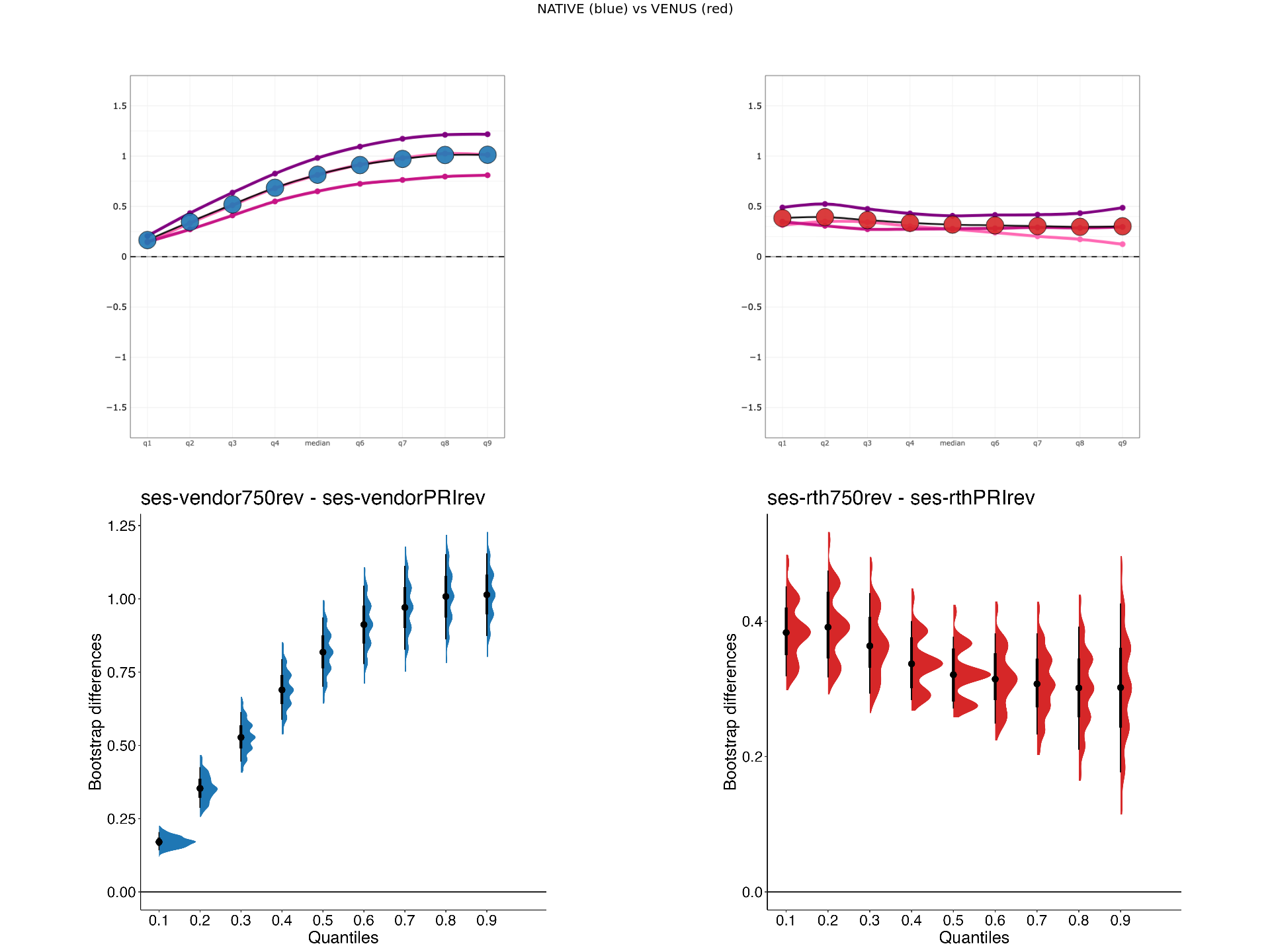
3.4.4Explore shift functions in pairs
[1] "../data/venus-data/qMRFlow/sub-invivo3/MTS_SF_PLOTS/sub-invivo3_rthPRIvsrth750_MTsat_rev.png"
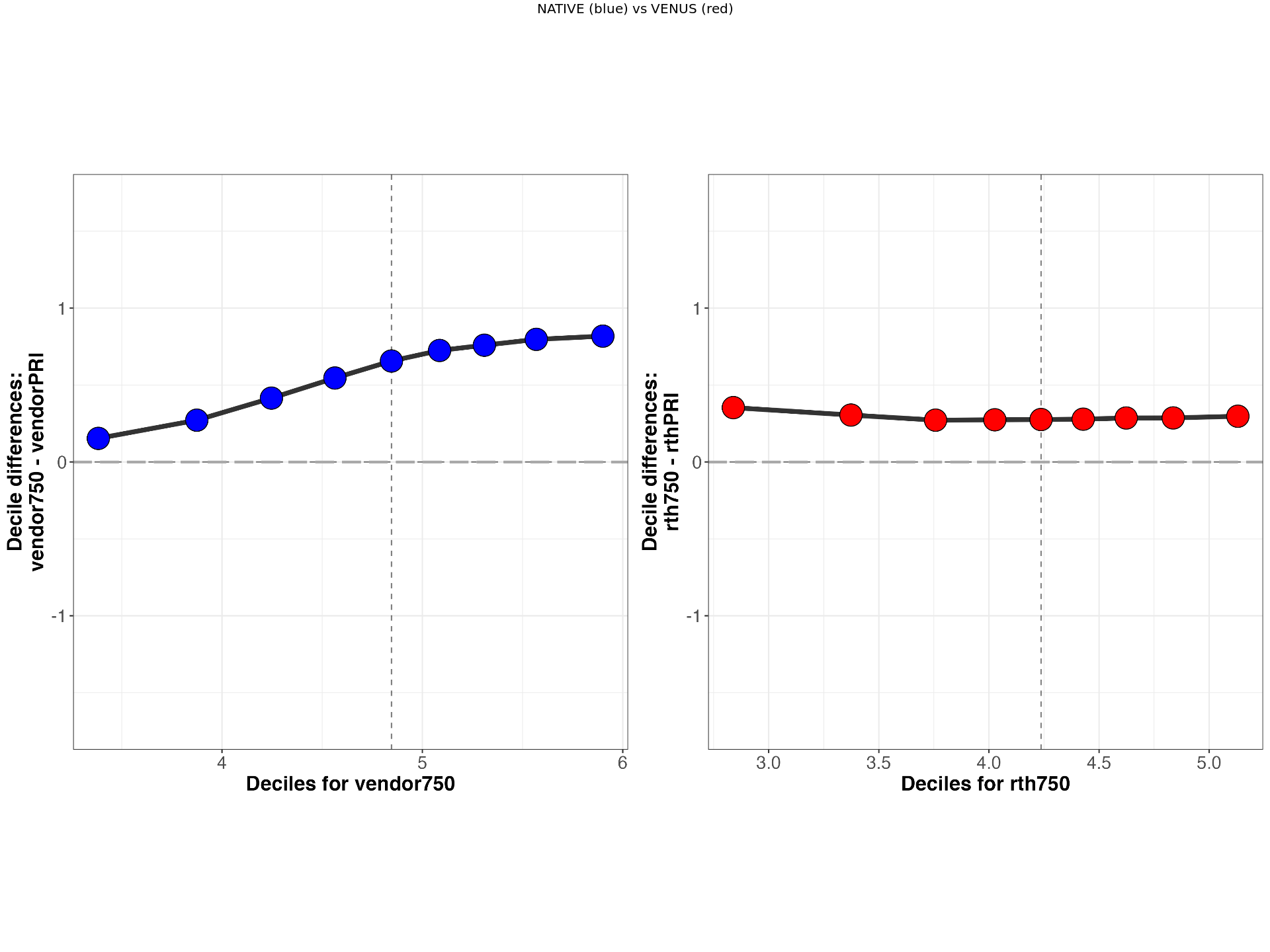
VENUS vs NATIVE comparision of MTsat values from Participant 3 for Siemens (S1) and GE (G1) scanners.
3.4.5Explore HSF plots

Explanation of the hierarchical shift function analysis.
[1] "../data/venus-data/HSF/rth750vsrthPRI_HSF_MTsat.png"
VENUS vs NATIVE comparision of MTsat values across participants for Siemens (S1) and GE (G1) scanners.
3.4.6Significance test
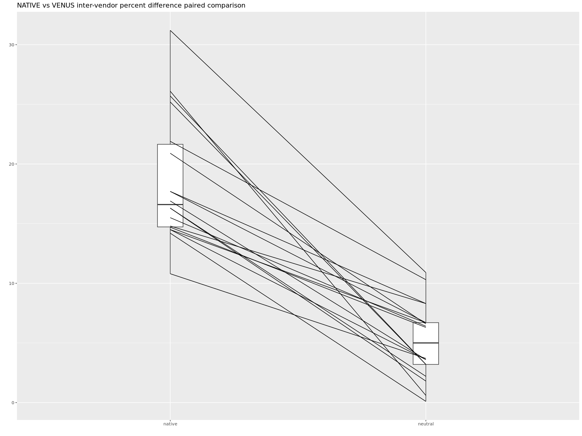
Paired comparison of difference scores between VENUS and NATIVE implementations.
4🏁 Conclusion
We conclude that vendor-neutral workflows are feasible and compatible with clinical MRI scanners. The significant reduction of inter-vendor variability using vendor-neutral sequences has important implications for qMRI research and for the reliability of multicenter clinical trials.
Acknowledgments
This research was undertaken thanks, in part, to funding from the Canada First ResearchExcellence Fund through the TransMedTech Institute. The work is also funded in part by theMontreal Heart Institute Foundation, Canadian Open Neuroscience Platform (Brain CanadaPSG), Quebec Bio-imaging Network (NS, 8436-0501 and JCA, 5886, 35450), Natural Sciencesand Engineering Research Council of Canada (NS, 2016-06774 and JCA, RGPIN-2019-07244),Fonds de Recherche du Québec (JCA, 2015-PR-182754), Fonds de Recherche du Québec- Santé (NS, FRSQ-36759, FRSQ-35250 and JCA, 28826), Canadian Institute of HealthResearch (JCA, FDN-143263 and GBP, FDN-332796), Canada Research Chair in QuantitativeMagnetic Resonance Imaging (950-230815), CAIP Chair in Health Brain Aging, CourtoisNeuroMod project and International Society for Magnetic Resonance in Medicine (ISMRMResearch Exchange Grant).
- Karakuzu, A., Biswas, L., Cohen-Adad, J., & Stikov, N. (2022). Vendor-neutral sequences and fully transparent workflows improve inter-vendor reproducibility of quantitative MRI. Magnetic Resonance in Medicine, 88(3), 1212–1228.
- Karakuzu, A., Biswas, L., Cohen‐Adad, J., & Stikov, N. (2022). Vendor‐neutral sequences and fully transparent workflows improve inter‐vendor reproducibility of quantitative <scp>MRI</scp>. Magnetic Resonance in Medicine, 88(3), 1212–1228. 10.1002/mrm.29292
- Cashmore, M. T., McCann, A. J., Wastling, S. J., McGrath, C., Thornton, J., & Hall, M. G. (2021). Clinical quantitative MRI and the need for metrology. The British Journal of Radiology, 94(1120). 10.1259/bjr.20201215
- Karakuzu, A., Blostein, N., Caron, A. V., Boré, A., Rheault, F., Descoteaux, M., & Stikov, N. (2025). Rethinking MRI as a measurement device through modular and portable pipelines. Magnetic Resonance Materials in Physics, Biology and Medicine, 1–17. 10.1007/s10334-025-01245-3
- Karakuzu, A., Appelhoff, S., Auer, T., Boudreau, M., Feingold, F., Khan, A. R., Lazari, A., Markiewicz, C., Mulder, M., Phillips, C., & others. (2022). qMRI-BIDS: An extension to the brain imaging data structure for quantitative magnetic resonance imaging data. Scientific Data, 9(1), 517. 10.1038/s41597-022-01658-x
- Karakuzu, A., Biswas, L., Cohen-Adad, J., & Stikov, N. (2021). Vendor-neutral sequences and fully transparent workflows improve inter-vendor reproducibility of quantitative MRI. 10.1101/2021.12.27.474259