Vendor-neutral sequences and their implications for the reproducibility of quantitative MRI
Shift function analysis
Shift function analysis
Source
options(warn = -1)
library(rogme)
library(tibble)
library(ggplot2)
library(R.matlab)
library(plotly)
library(htmlwidgets)
library(tidyverse)
library(plyr)
library(dplyr)
library(png)
library(grid)
library(gridExtra)
library(repr)
library(PairedData)
set.seed(123)

percentage_difference <- function(value, value_two) {
  pctd = abs(value - value_two) / ((value + value_two) / 2) * 100
  return(pctd)
}

obj2plotly <- function(curObj,acq,plim){

if (acq=="rth"){
color="#d62728"
}else{
color="#1f77b4"
}

p<-plot_hsf_pb(curObj, viridis_option="D", ind_line_alpha=0.9, ind_line_size=1, gp_line_colour = "red", gp_point_colour=color,gp_point_size=4,gp_line_size=1.5)
p$labels$colour = ""
p$data$participants = revalue(p$data$participants,c("1"="sub1", "2"="sub2","3"="sub3"))

th <- ggplot2::theme_bw() + ggplot2::theme(
  legend.title = element_blank(),
  axis.line=element_blank(),
    legend.position = "none",
  axis.ticks = element_blank(),
  #axis.text = element_blank(),
  axis.title = element_blank(),
  panel.border = element_rect(colour = "black", fill=NA, size=0.5)
  )

k <-p  + th + aes(x = dec, y = diff, colour = participants) + ggtitle("")

k$labels$colour = revalue(k$labels$colour,c("red"="group"))

axx <- list(
  zeroline = FALSE,
  tickmode = "array",
  tickvals = c("0.1","0.2","0.3","0.4","0.5","0.6","0.7","0.8","0.9"),
  ticktext = c("q1","q2","q3","q4","median","q6","q7","q8","q9"),
  showticklabels= TRUE,
  ticksuffix=" "
)

axy <- list(
  zeroline = FALSE,
  range = c(-plim,plim),
  overlaying = "y2",
  showticklabels= FALSE
  # The range is fixed per panel (3 MAD from both side) to infer the relative effect size
)

axy2 <- list(
  range = c(-plim,plim),
    showticklabels= TRUE,
    ticksuffix=" "
  # The range is fixed per panel (3 MAD from both side) to infer the relative effect size
)
figObj <- ggplotly(k) %>%
            layout(height=800,width=800,xaxis=axx,yaxis = axy, yaxis2 = axy2, margin=c(5,5,5,5)) %>% # SWITCH BACK TO 400 x 400
            style(traces=1,mode="lines+markers",opacity=1,marker=list(size=10),line = list(shape = "spline",color="purple",width=5)) %>%
            style(traces=2,mode="lines+markers",opacity=1,marker=list(size=10),line = list(shape = "spline",color="hotpink",width=5)) %>%
            style(traces=3,mode="lines+markers",opacity=1,marker=list(size=10),line = list(shape = "spline",color="mediumvioletred",width=5)) %>%
            style(traces=4,opacity=1,line = list(color="black",width=2,dash="dash"),yaxis = 'y2') %>% # zero line
            style(traces=5,mode = "lines+markers",opacity=0.9,line = list(shape = "spline",width=3,color="black"),marker = list(color=color,size=30,line=list(color="black",width=1))) %>% # group markers
            style(traces=6,opacity=0,line = list(shape = "spline",color="#762a83",width=3))
return(figObj)
} #END FUNCTION DEF

get_vector <- function(subject, session, metric, nSamples,derivativesDir){
  derivativesDir <- paste(derivativesDir,subject ,"/",sep = "")
  curMat <- readMat(paste(derivativesDir,session,"/stat/",subject,"_",session,"_desc-wm_metrics.mat",sep = ""))
  curMetric <- curMat[[metric]]
  if (metric == "MTR"){
      curMetric <- curMetric[!sapply(curMetric, is.nan)]
      curMetric <- curMetric[curMetric > 35]
      curMetric <- curMetric[curMetric < 70]
  }else if (metric == "MTsat"){
      curMetric <- curMetric[!sapply(curMetric, is.nan)]
      curMetric <- curMetric[curMetric > 1]
      curMetric <- curMetric[curMetric < 8]
  }else if (metric == "T1"){
      curMetric <- curMetric[!sapply(curMetric, is.nan)]
      curMetric <- curMetric[curMetric > 0]
      curMetric <- curMetric[curMetric < 3]
  }
  curMetric <- sample (curMetric, size=nSamples, replace =F)
  return(curMetric)
} #END FUNCTION DEF

get_df <- function(ses1,ses2,metric,nSamples){
df2 <- tibble(participant=as_factor(c(rep(1,nSamples*2),rep(2,nSamples*2),rep(3,nSamples*2))))
df2["condition"] = as_factor(rep(c(rep(ses1,nSamples),rep(ses2,nSamples)),3))
curComp = c(get_vector("sub-invivo1",ses1,metric,nSamples,derivativesDir),
       get_vector("sub-invivo1",ses2,metric,nSamples,derivativesDir),
       get_vector("sub-invivo2",ses1,metric,nSamples,derivativesDir),
       get_vector("sub-invivo2",ses2,metric,nSamples,derivativesDir),
       get_vector("sub-invivo3",ses1,metric,nSamples,derivativesDir),
       get_vector("sub-invivo3",ses2,metric,nSamples,derivativesDir))
df2["metric"] = curComp
return(df2)
} #END FUNCTION DEF

display_sf <- function(derivativesDir,sub,scn1,scn2,metric,implementation){

    T1DIR = paste(derivativesDir,sub,"/","T1_SF_PLOTS",sep="")
    MTRDIR = paste(derivativesDir,sub,"/","MTR_SF_PLOTS",sep="")
    MTSDIR = paste(derivativesDir,sub,"/","MTS_SF_PLOTS",sep="")
    ses_venus=data.frame(row.names=c("G1","S1","S2") , val=c("rth750","rthPRI","rthSKY"))
    ses_native=data.frame(row.names=c("G1","S1","S2") , val=c("vendor750","vendorPRI","vendorSKY"))

    if (metric=="T1"){
        curDir = T1DIR
    }else if (metric=="MTR"){
        curDir = MTRDIR
    }else if (metric=="MTsat"){
        curDir = MTSDIR
    }

    sel1 = ses_venus[scn1,]
    sel2 = ses_venus[scn2,]

    file1 = paste(curDir,"/",sub,"_",sel1,"vs",sel2,"_",metric,"_rev.png",sep="")
    print(file1)
    file2 = paste(curDir,"/",sub,"_",sel2,"vs",sel1,"_",metric,"_rev.png",sep="")

    if (file.exists(file1)){
        plot1 <- readPNG(file2)
        plot2 <- readPNG(paste(curDir,"/",sub,"_",ses_native[scn1,],"vs",ses_native[scn2,],"_",metric,"_rev.png",sep=""))
        grid.arrange(rasterGrob(plot2),rasterGrob(plot1),nrow=1,top=textGrob(label="NATIVE (blue) vs VENUS (red)",size=12))
    }else if (file.exists(file2)){
        plot1 <- readPNG(file2)
        plot2 <- readPNG(paste(curDir,"/",sub,"_",ses_native[scn2,],"vs",ses_native[scn1,],"_",metric,"_rev.png",sep=""))
        grid.arrange(rasterGrob(plot2),rasterGrob(plot1),nrow=1,top=textGrob("NATIVE (blue) vs VENUS (red)"))
    }else {
        print("No file")
    }

}

display_hsf <- function(derivativesDir,scn1,scn2,metric){

    curDir = paste(derivativesDir,"HSF",sep="")
    ses_venus=data.frame(row.names=c("G1","S1","S2") , val=c("rth750","rthPRI","rthSKY"))
    ses_native=data.frame(row.names=c("G1","S1","S2") , val=c("vendor750","vendorPRI","vendorSKY"))

    sel1 = ses_venus[scn1,]
    sel2 = ses_venus[scn2,]

    file1 = paste(curDir,"/",sel1,"vs",sel2,"_HSF_",metric,".png",sep="")
    print(file1)
    file2 = paste(curDir,"/",sel2,"vs",sel1,"_HSF_",metric,".png",sep="")

    if (file.exists(file1)){
        plot1 <- readPNG(file1)
        plot2 <- readPNG( paste(curDir,"/",ses_native[scn1,],"vs",ses_native[scn2,],"_HSF_",metric,".png",sep=""))
        plot3 <- readPNG( paste(curDir,"/",ses_venus[scn1,],"vs",ses_venus[scn2,],"_HSFdif_",metric,".png",sep=""))
        plot4 <- readPNG( paste(curDir,"/",ses_native[scn1,],"vs",ses_native[scn2,],"_HSFdif_",metric,".png",sep=""))
        grid.arrange(rasterGrob(plot2),rasterGrob(plot1),rasterGrob(plot4),rasterGrob(plot3),nrow=2,ncol=2,top=textGrob("NATIVE (blue) vs VENUS (red)"))
    }else if (file.exists(file2)){
        plot1 <- readPNG(file2)
        plot2 <- readPNG( paste(curDir,"/",ses_native[scn2,],"vs",ses_native[scn1,],"_HSF_",metric,".png",sep=""))
        grid.arrange(rasterGrob(plot2),rasterGrob(plot1),nrow=1,top=textGrob("NATIVE (blue) vs VENUS (red)"))
    }else {
        print("No file")
    }

}


derivativesDir <- "../data/venus-data/qMRFlow/"

subs = list("sub-invivo1","sub-invivo2","sub-invivo3")
metrics = list("T1","MTR","MTsat")
sessions <- list("ses-rth750rev","ses-rthPRIrev","ses-rthSKYrev","ses-vendor750rev","ses-vendorPRIrev","ses-vendorSKYrev")

options(repr.plot.width=16, repr.plot.height=12)
Output
R.matlab v3.7.0 (2022-08-25 21:52:34 UTC) successfully loaded. See ?R.matlab for help.
Attaching package: ‘R.matlab’
The following objects are masked from ‘package:base’:

    getOption, isOpen
Attaching package: ‘plotly’
The following object is masked from ‘package:ggplot2’:

    last_plot
The following object is masked from ‘package:stats’:

    filter
The following object is masked from ‘package:graphics’:

    layout
── Attaching core tidyverse packages ──────────────────────── tidyverse 2.0.0 ──
✔ dplyr     1.1.4     ✔ readr     2.1.5
✔ forcats   1.0.0     ✔ stringr   1.5.1
✔ lubridate 1.9.4     ✔ tidyr     1.3.1
✔ purrr     1.0.2
── Conflicts ────────────────────────────────────────── tidyverse_conflicts() ──
✖ dplyr::filter() masks plotly::filter(), stats::filter()
✖ dplyr::lag()    masks stats::lag()
ℹ Use the conflicted package (<http://conflicted.r-lib.org/>) to force all conflicts to become errors
------------------------------------------------------------------------------
You have loaded plyr after dplyr - this is likely to cause problems.
If you need functions from both plyr and dplyr, please load plyr first, then dplyr:
library(plyr); library(dplyr)
------------------------------------------------------------------------------
Attaching package: ‘plyr’
The following objects are masked from ‘package:dplyr’:

    arrange, count, desc, failwith, id, mutate, rename, summarise,
    summarize
The following object is masked from ‘package:purrr’:

    compact
The following objects are masked from ‘package:plotly’:

    arrange, mutate, rename, summarise
Attaching package: ‘gridExtra’
The following object is masked from ‘package:dplyr’:

    combine
Loading required package: MASS
Attaching package: ‘MASS’
The following object is masked from ‘package:dplyr’:

    select
The following object is masked from ‘package:plotly’:

    select
Loading required package: gld
Loading required package: mvtnorm
Loading required package: lattice
Attaching package: ‘PairedData’
The following object is masked from ‘package:base’:

    summary
T1, MTR and MTSat shift function analysis
The following code cell performs a percentile bootstrapped comparison of dependent samples using Harrell-Davis quantile estimator. Outputs will be written as png and csv files to the following directories:
.../qMRFLow/sub-invivo#/T1_SF_PLOTSfor T1 comparisons.../qMRFLow/sub-invivo#/MTR_SF_PLOTSfor MTR comparisons.../qMRFLow/sub-invivo#/MTS_SF_PLOTSfor MTsat comparisons
Source
# metrics = list("MTR","T1","MTsat")
# for (metric in metrics){
# for (sub in subs) {

# T1DIR = paste(derivativesDir,sub,"/","T1_SF_PLOTS",sep="")
# MTRDIR = paste(derivativesDir,sub,"/","MTR_SF_PLOTS",sep="")
# MTSDIR = paste(derivativesDir,sub,"/","MTS_SF_PLOTS",sep="")
# dir.create(T1DIR)
# dir.create(MTRDIR)
# dir.create(MTSDIR)

# sessions <- list("ses-rth750rev","ses-rthPRIrev","ses-rthSKYrev","ses-vendor750rev","ses-vendorPRIrev","ses-vendorSKYrev")

# # Create dataframe with 37k samples per session
# nSamples = 37000
# df <- tibble(N = 1:nSamples)
# for (i in seq(from=1, to=length(sessions), by=1)) {
#   curMat <- readMat(paste(derivativesDir,sub,"/",sessions[i],"/stat/",sub,"_",sessions[i],"_desc-wm_metrics.mat",sep = ""))
#   curMetric <- curMat[[metric]]
#   if (metric == "MTR"){
#       OUTDIR = MTRDIR
#       PLTRANGE = 10.1
#       curMetric <- curMetric[curMetric > 35]
#       curMetric <- curMetric[curMetric < 70]
#   }else if (metric == "MTsat"){
#       OUTDIR = MTSDIR
#       PLTRANGE = 1.7
#       curMetric <- curMetric[curMetric > 1]
#       curMetric <- curMetric[curMetric < 8]
#   }else if (metric == "T1"){
#       OUTDIR = T1DIR
#       PLTRANGE = 0.5
#       curMetric <- curMetric[curMetric > 0]
#       curMetric <- curMetric[curMetric < 3]
#   }
#   # Do not choose the same element more than once
#   print(length(curMetric))
#   curMetric <- sample (curMetric, size=nSamples, replace =F)
#   varName <- toString(sessions[i])
#   varName <- substr(varName,5,nchar(varName)-3)
#   print(varName)
#   df <- mutate(df, !!varName := curMetric)
# }

# neutral = list("rth750","rthPRI","rthSKY")
# native  = list("vendor750","vendorPRI","vendorSKY")
# combns <- combn(c(1,2,3),2)

# for (j in seq(from=1,to=2, by=1)){
# for (i in seq(from=1,to=3, by=1)){

# if (j==1){
#     sel1 = toString(neutral[combns[,i][1]])
#     sel2 = toString(neutral[combns[,i][2]])
#     }
# else
# {
#     sel1 = toString(native[combns[,i][1]])
#     sel2 = toString(native[combns[,i][2]])
# }

# paste(sel1,"vs",sel2," T1",' in progress',sep="")

# grp1 <- df[[sel1]]
# grp2 <- df[[sel2]]

# sfInput <- mkt2(grp1,grp2,group_labels=c(sel1,sel2))
# sf <- shiftdhd_pbci(
#   data = sfInput,
#   formula = obs ~ gr,
#   nboot = 250,
#   alpha = 0.05/30
# )

# sf[[1]]['pctdif'] = percentage_difference(sf[[1]][[sel1]],sf[[1]][[sel2]])
# write.csv(sf,paste(OUTDIR,"/",sub,"_",sel1,"vs",sel2,"_",metric,"_rev",'.csv',sep=""))
# print(min(percentage_difference(sf[[1]][[sel1]],sf[[1]][[sel2]])))
# print(percentage_difference(sf[[1]][[sel1]],sf[[1]][[sel2]])[5])
# print(max(percentage_difference(sf[[1]][[sel1]],sf[[1]][[sel2]])))

# th <- ggplot2::theme_dark() + ggplot2::theme(
#   panel.border = element_blank(),
#   panel.background = element_rect(fill = "black"),
#   plot.background = element_rect(fill = "black"),
#   legend.background = element_rect(fill="white",size=0.5),
#   legend.text=element_text(color="white",size=12),
#   axis.line=element_blank(),
#   axis.text = element_blank(),
#   axis.title = element_blank(),
#   axis.text.x = element_text(colour="white",size=18,face='bold'),
#   axis.text.y = element_text(colour="white",size=18,face='bold')
#   )

# if (j==1){
#     lnclr = "darkgray"
#     flclr = "red"
# } else
# {
#     lnclr = "darkgray"
#     flclr = "blue"
# }

# psf <- plot_sf(
#   data = sf,
#   plot_theme = 1,
#   symb_col = "black",
#   symb_fill = flclr,
#   symb_size = 8,
#   symb_shape = 21,
#   diffint_col = "white",
#   diffint_size = 1.5,
#   q_line_col = "black",
#   q_line_alpha = 0.8,
#   q_line_size = 1.8,
#   theme2_alpha = NULL
# )

# curPlot <- psf[[1]] + geom_hline(yintercept = 0,colour=lnclr, linetype = "longdash",size=1) + ylim(-PLTRANGE,PLTRANGE)
# ggsave(
#   filename = paste(OUTDIR,"/",sub,"_",sel1,"vs",sel2,"_",metric,"_rev",'.png',sep=""),
#   plot = curPlot,
#   device = NULL,
#   path = NULL,
#   scale = 1,
#   width = NA,
#   height = NA,
#   units = c("mm"),
#   dpi = 300,
#   limitsize = TRUE
# )
# }}
# }}1Explore shift function plots
Source
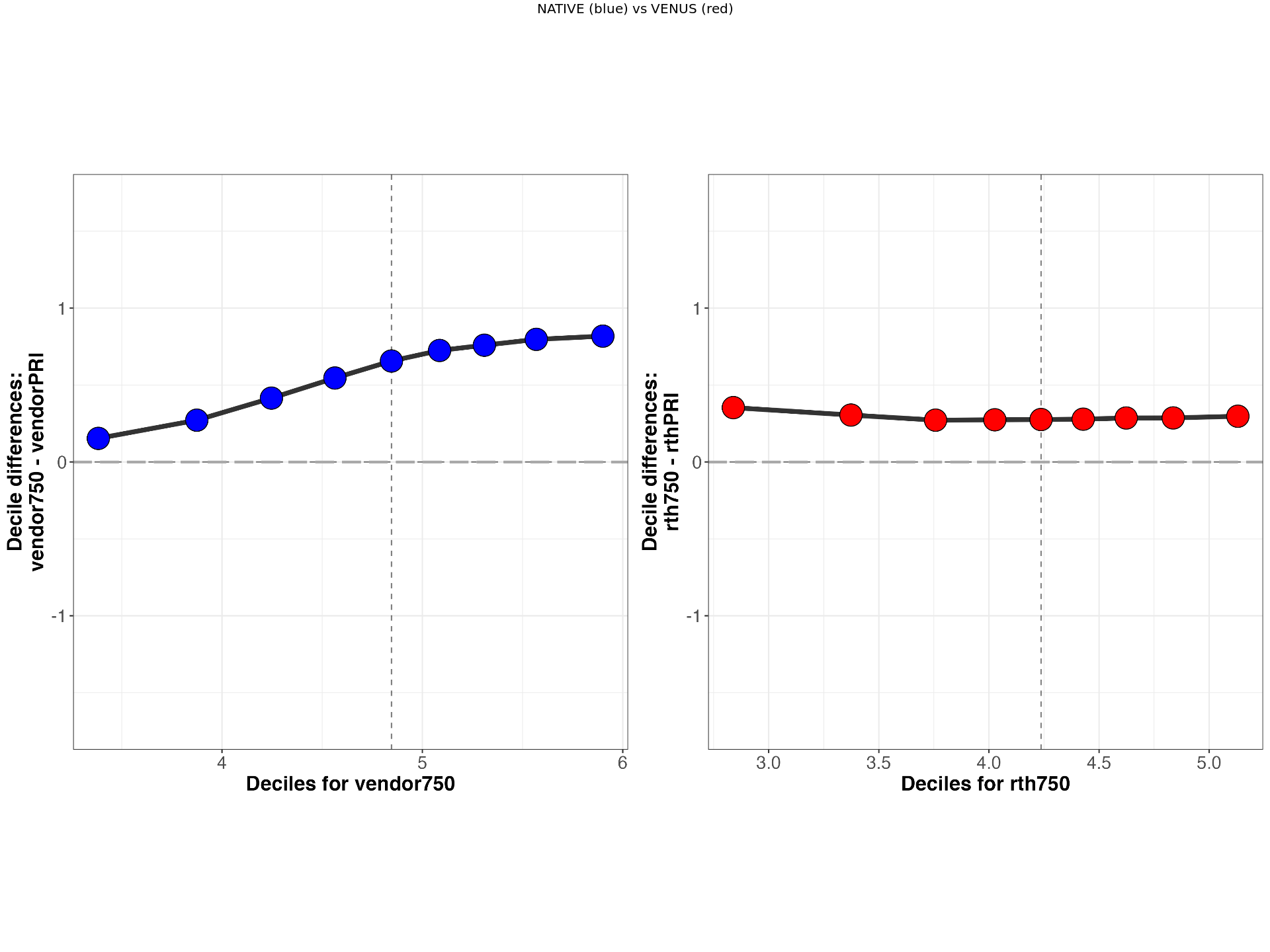
subject ="sub-invivo3" # or sub-invivo2 or sub-invivo3
metric ="MTsat" # or MTR or MTsat
scanner1 = "S1" # or S1 or S2
scanner2 = "G1" # or G1 or S2


display_sf(derivativesDir,subject,scanner1,scanner2,metric,implementation)
[1] "../data/venus-data/qMRFlow/sub-invivo3/MTS_SF_PLOTS/sub-invivo3_rthPRIvsrth750_MTsat_rev.png"
Perform hierarchical shift function (HSF) analysis
The following code cell iterates over all the comparisons and saves interactive HSF figures.
.../HSF
Source
# HSFDIR = paste(derivativesDir,"HSF/",sep="")
# #HSFDIR = paste("HSF/",sep="")
# dir.create(HSFDIR)

# sessions <- list("ses-rth750rev","ses-rthPRIrev","ses-rthSKYrev","ses-vendor750rev","ses-vendorPRIrev","ses-vendorSKYrev")
# nSamples = 37000

# neutral = list("ses-rth750rev","ses-rthPRIrev","ses-rthSKYrev")
# native  = list("ses-vendor750rev","ses-vendorPRIrev","ses-vendorSKYrev")
# combns <- combn(c(1,2,3),2)

# metrics = list("T1","MTR","MTsat")
# for (metric in metrics){

# if (metric == "MTR"){
#       PLTRANGE = 10.3
#   }else if (metric == "MTsat"){
#       PLTRANGE = 1.8
#   }else if (metric == "T1"){
#       PLTRANGE = 0.6
#   }
# for (j in seq(from=1,to=2, by=1)){
# for (i in seq(from=1,to=3, by=1)){

# if (j==1){
#     sel1 = toString(neutral[combns[,i][1]])
#     sel2 = toString(neutral[combns[,i][2]])
#     clr = "rth"
#     }
# else
# {
#     clr = "vendor"
#     sel1 = toString(native[combns[,i][1]])
#     sel2 = toString(native[combns[,i][2]])
# }

# print(paste(sel1,"vs",sel2," T1",' in progress',sep=""))
# cur_df <-get_df(sel1,sel2,metric,nSamples)
# out <- hsf_pb(
#   data = cur_df,
#   formula = metric ~ condition + participant,
#   qseq = seq(0.1, 0.9, 0.1),
#   tr = 0,
#   alpha = 0.05,
#   qtype = 8,
#   todo = c(1, 2),
#   nboot = 750)
# htmlwidgets::saveWidget(obj2plotly(out,clr,PLTRANGE), file = paste(substr(sel1,5,nchar(sel1)-3),"vs",substr(sel2,5,nchar(sel2)-3),"_HSF_",metric,".html",sep=""))
# }}}
Source
metric ="MTsat" # or MTR or T1
scanner1 = "G1" # or S1 or S2
scanner2 = "S1" # or G1 or S2


display_hsf("../data/venus-data/",scanner1,scanner2,metric)
[1] "../data/venus-data/HSF/rth750vsrthPRI_HSF_MTsat.png"
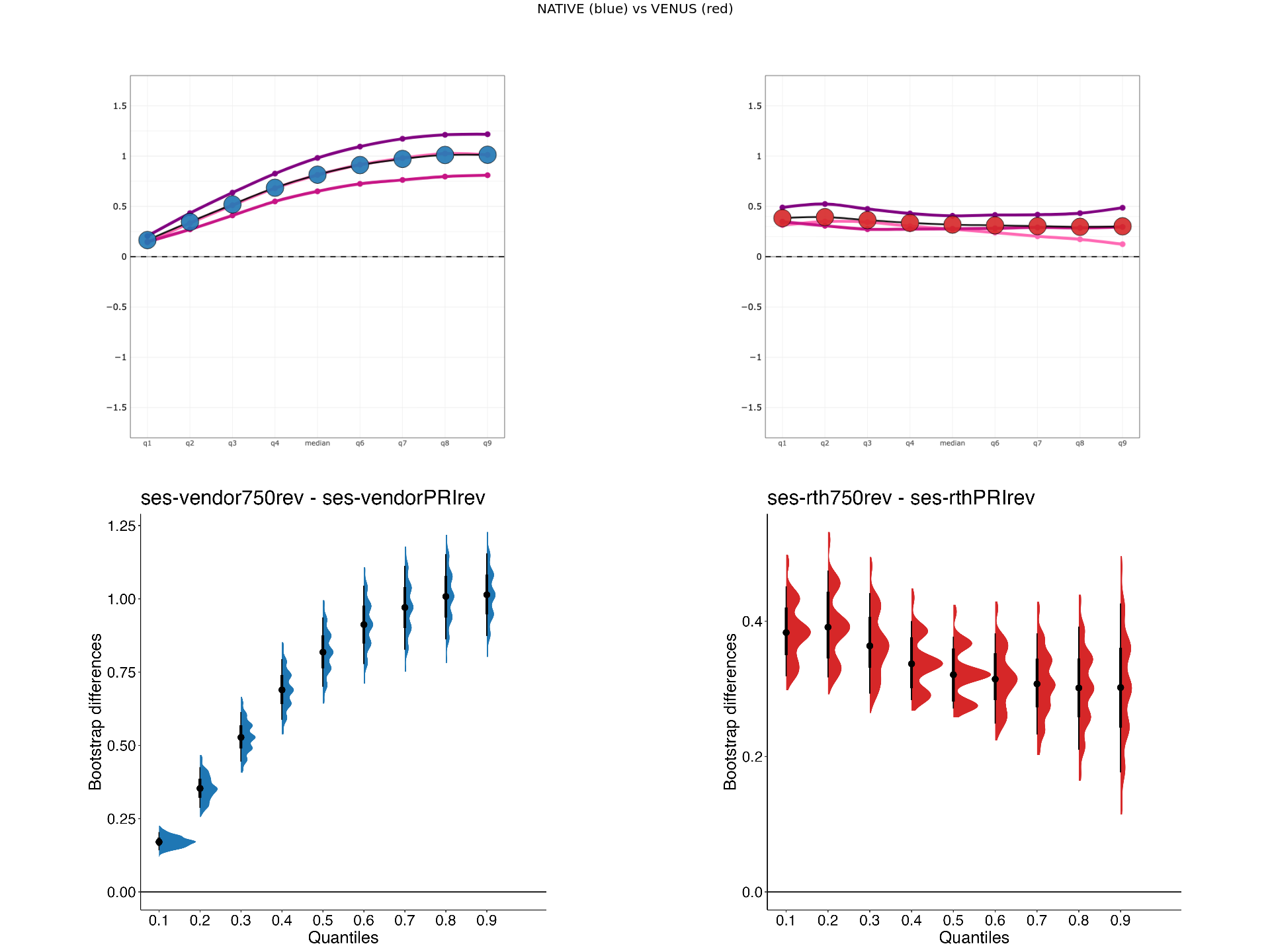
Bootstrapped differences at each decile for HSF
Source
# HSFDIR = paste(derivativesDir,"HSF/",sep="")
# dir.create(HSFDIR)

# sessions <- list("ses-rth750rev","ses-rthPRIrev","ses-rthSKYrev","ses-vendor750rev","ses-vendorPRIrev","ses-vendorSKYrev")
# nSamples = 37000

# neutral = list("ses-rth750rev","ses-rthPRIrev","ses-rthSKYrev")
# native  = list("ses-vendor750rev","ses-vendorPRIrev","ses-vendorSKYrev")
# combns <- combn(c(1,2,3),2)

# metrics = list("T1","MTR","MTsat")
# for (metric in metrics){

# if (metric == "MTR"){
#       PLTRANGE = 10.3
#   }else if (metric == "MTsat"){
#       PLTRANGE = 1.8
#   }else if (metric == "T1"){
#       PLTRANGE = 0.6
#   }
# for (j in seq(from=1,to=2, by=1)){
# for (i in seq(from=1,to=3, by=1)){

# if (j==1){
#     sel1 = toString(neutral[combns[,i][1]])
#     sel2 = toString(neutral[combns[,i][2]])
#     clr = "#d62728"
#     }
# else
# {
#     clr = "#1f77b4"
#     sel1 = toString(native[combns[,i][1]])
#     sel2 = toString(native[combns[,i][2]])
# }

# print(paste(sel1,"vs",sel2," T1",' in progress',sep=""))


# cur_df <-get_df(sel1,sel2,metric,nSamples)
# out <- hsf_pb(
#   data = cur_df,
#   formula = metric ~ condition + participant,
#   todo = c(1, 2),
#   nboot = 750)
# obj <- plot_hsf_pb_dist(out,fill_colour=clr,point_interv="median")
# ggsave(
#   filename = paste(substr(sel1,5,nchar(sel1)-3),"vs",substr(sel2,5,nchar(sel2)-3),"_HSFdif_",metric,".png",sep=""),
#   plot = obj,
#   device = NULL,
#   path = NULL,
#   scale = 1,
#   width = NA,
#   height = NA,
#   units = c("mm"),
#   dpi = 300,
#   limitsize = TRUE
# )
# #orca(obj, file = paste(substr(sel1,5,nchar(sel1)-3),"vs",substr(sel2,5,nchar(sel2)-3),"_HSFdif_",metric,".png",sep=""))
# }}}
Significance test
Paired comparison of difference scores between VENUS and NATIVE implementations.
Source
data <- data.frame(participant = rep(1:3, each=12),
                   sequence = rep(c("native","venus"), times=18),
                   metric = rep(c("T1","T1","T1","T1","MTR","MTR","MTR", "MTR","MTsat","MTsat","MTsat", "MTsat"),3),
                   pctdif = c(31.2,10.9,16.30,1.8,17.7,8.3,16.9,3.6,14.5,6.7,25.7,3.2,
                             20.9,6.6,10.8,3.7,15.5,6.4,14.8,8.3,17.7,6.7,25.2,3.2,
                            14.2,0.1,14.5,3.6,14.7,6.3,16.3,2.2,21.9,10.3,26.1,0.6))

# group_by(data, sequence) %>%
#   dplyr::summarise(
#     count = n(),
#     median = median(pctdif, na.rm = TRUE),
#     IQR = IQR(pctdif, na.rm = TRUE)
#   )


neutral <- data$pctdif[data$sequence=="venus"]
native <- data$pctdif[data$sequence=="native"]
pd <- paired(native,neutral)
plt <- plot(pd, type = "profile") + ggtitle("NATIVE vs VENUS inter-vendor percent difference paired comparison") + theme_gray()
# Plotly outputs will not be rendered in Jupyter Book.
# ggplotly(plt)
plt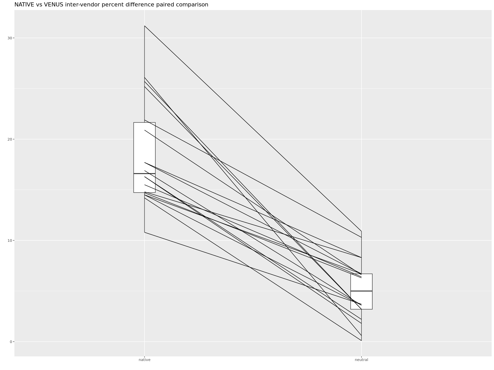
Source
# Across scores
res <- wilcox.test(pctdif ~ sequence,data=data, paired=TRUE)
p.adjust(res$p.value, method = "BH", n = 6*3)
print('Across metrics significance')
print(res)
# T1
res <- wilcox.test(subset(data,sequence=="native" & metric=="T1")$pctdif,subset(data,sequence=="venus" & metric=="T1")$pctdif,paired=TRUE,alternative = "greater")
print('T1 significance before correction')
print(res)
print('T1 significance after correction')
p.adjust(res$p.value, method = "bonferroni", n = 3)


# MTR
res <- wilcox.test(subset(data,sequence=="native" & metric=="MTR")$pctdif,subset(data,sequence=="venus" & metric=="MTR")$pctdif,paired=TRUE,alternative = "greater")
print('MTR significance before correction')
print(res)
print('MTR significance after correction')
p.adjust(res$p.value, method = "bonferroni", n = 3)

# MTsat
res <- wilcox.test(subset(data,sequence=="native" & metric=="MTsat")$pctdif,subset(data,sequence=="venus" & metric=="MTsat")$pctdif,paired=TRUE,alternative = "greater")
print('MTsat significance before correction')
print(res)
print('MTsat significance after correction')
p.adjust(res$p.value, method = "bonferroni", n = 3)
Loading...
- Karakuzu, A., Biswas, L., Cohen-Adad, J., & Stikov, N. (2021). Vendor-neutral sequences and fully transparent workflows improve inter-vendor reproducibility of quantitative MRI. 10.1101/2021.12.27.474259