Results: dataset level
Contents
import warnings

warnings.filterwarnings("ignore")

import ipywidgets as widgets
from ipywidgets import interactive
from fmriprep_denoise.visualization import utils


path_root = utils.repo2data_path() / "denoise-metrics"

strategy_order = list(utils.GRID_LOCATION.values())
group_order = {
    "ds000228": ["adult", "child"],
    "ds000030": ["control", "ADHD", "bipolar", "schizophrenia"],
}
datasets = ["ds000228", "ds000030"]

datasets_baseline = {"ds000228": "adult", "ds000030": "control"}
---- repo2data starting ----
/srv/conda/envs/notebook/lib/python3.8/site-packages/repo2data
Config from file :
/home/jovyan/binder/data_requirement.json
Destination:
../../data/fmriprep-denoise-benchmark

Info : ../../data/fmriprep-denoise-benchmark already downloaded
Results: dataset level#
Important
The dropdown menu only works in interactive mode! Please launch binder to see the alterative results.
Here we provides alternative visualisation of the benchmark results from the manuscript. Please click on the launch button to lunch the Binder instance for interactive data viewing.
The benchmark was performed on two Long-Term Support (LTS) versions of fMRIPrep (20.2.1 and 20.2.5) and two OpenNeuro datasets (ds000228 [Richardson et al., 2019] and ds000030 [Bilder et al., 2020]).
For the demographic information and gross mean framewise displacement, it is possible to generate the report based on three levels of quality control filters (no filter, minimal, stringent).
Sample and subgroup size change based on quality control criteria#
We would like to perform the benchmark on subjects with reasonable qulaity of data to reflect the decisions researchers make in data analysis. We modified the criteria for filtering data from [Parkes et al., 2018] to suit our dataset better and ensure enough time points for functional connectivity analysis.
The stringent threshold removes subjects based on two criteria:
removes subjects with mean framewise displacement above 0.25 mm
removes subjects with more than 80% of the volumes missing when filtering the time series with a 0.2 mm framewise displacement.
Parkes and colleagues [Parkes et al., 2018] used a stricter criteria for remaining volumes (20%). However this will removed close to or more than 50% of the subjects from the datasets.
In addition, we included the minimal threshold from [Parkes et al., 2018] (removes subjects with mean framewise displacement above 0.55 mm) for readers to expore.
import pandas as pd
from fmriprep_denoise.visualization import tables
from fmriprep_denoise.features.derivatives import get_qc_criteria


def demographic_table(criteria_name, fmriprep_version):
    criteria = get_qc_criteria(criteria_name)
    ds000228 = tables.lazy_demographic(
        "ds000228", fmriprep_version, path_root, **criteria
    )
    ds000030 = tables.lazy_demographic(
        "ds000030", fmriprep_version, path_root, **criteria
    )

    desc = pd.concat(
        {"ds000228": ds000228, "ds000030": ds000030}, axis=1, names=["dataset"]
    )
    desc = desc.style.set_table_attributes('style="font-size: 12px"')
    print("Generating new tables...")

    display(desc)


criteria_name = widgets.Dropdown(
    options=["stringent", "minimal", None],
    value="stringent",
    description="Threshould: ",
    disabled=False,
)
fmriprep_version = widgets.Dropdown(
    options=["fmriprep-20.2.1lts", "fmriprep-20.2.5lts"],
    value="fmriprep-20.2.1lts",
    description="Preporcessing version : ",
    disabled=False,
)
interactive(
    demographic_table, criteria_name=criteria_name, fmriprep_version=fmriprep_version
)
You can also use different exclusion criteria to explore the motion profiles of different subgroups in the dataset.
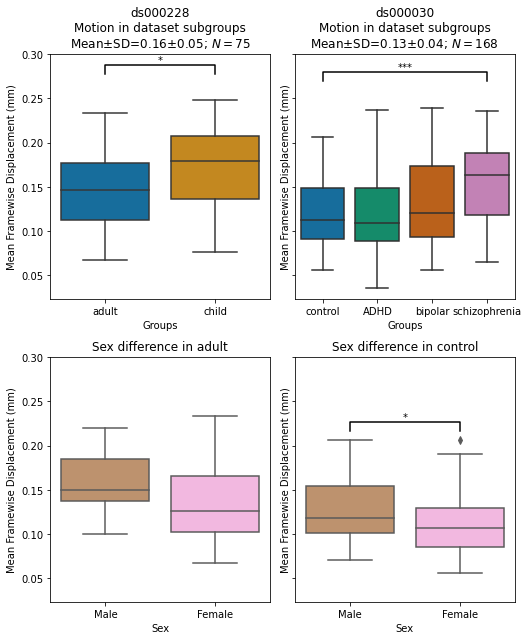
Motion profile of each dataset#
We can see overall the adults have less gross motion than children in ds000228.
Between different clinical groups in ds000030, the schizophrania group displays a marked difference in motion comparing to the healthy control.
from fmriprep_denoise.visualization import mean_framewise_displacement


def notebook_plot_mean_fd(criteria_name, fmriprep_version):
    stats = mean_framewise_displacement.load_data(
        path_root, criteria_name, fmriprep_version
    )
    mean_framewise_displacement.plot_stats(stats)


criteria_name = widgets.Dropdown(
    options=["stringent", "minimal", None],
    value="stringent",
    description="Threshould: ",
    disabled=False,
)
fmriprep_version = widgets.Dropdown(
    options=["fmriprep-20.2.1lts", "fmriprep-20.2.5lts"],
    value="fmriprep-20.2.1lts",
    description="Preporcessing version : ",
    disabled=False,
)
interactive(
    notebook_plot_mean_fd,
    criteria_name=criteria_name,
    fmriprep_version=fmriprep_version,
)
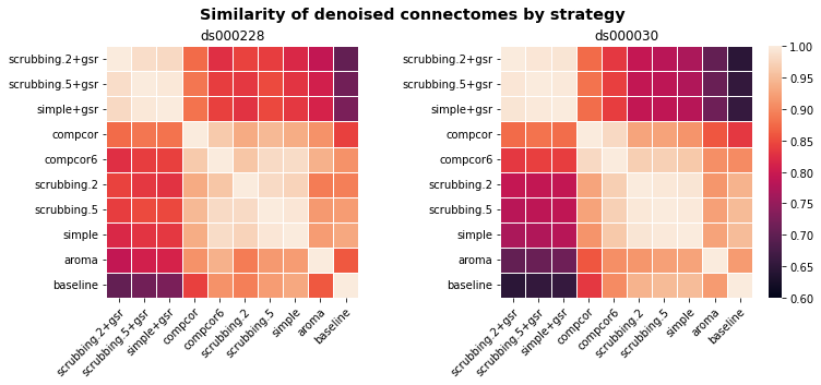
Similarity amongst denoised connectomes#
We plotted the correlations among connectomes denoised with different denoisng strategies to get a general sense of the data.
We see connectome denoised with or without global signal regressor formed two separate clusters. The baseline and ICA-AROMA [Pruim et al., 2015] denoised connectome do not belong to any clusters. ICA-AROMA potentially captures much more different source of noise than the others.
from fmriprep_denoise.visualization import connectivity_similarity


def notebook_plot_connectomes(fmriprep_version):
    average_connectomes = connectivity_similarity.load_data(
        path_root, datasets, fmriprep_version
    )
    connectivity_similarity.plot_stats(average_connectomes)


fmriprep_version = widgets.Dropdown(
    options=["fmriprep-20.2.1lts", "fmriprep-20.2.5lts"],
    value="fmriprep-20.2.1lts",
    description="Preporcessing version : ",
    disabled=False,
)
interactive(notebook_plot_connectomes, fmriprep_version=fmriprep_version)
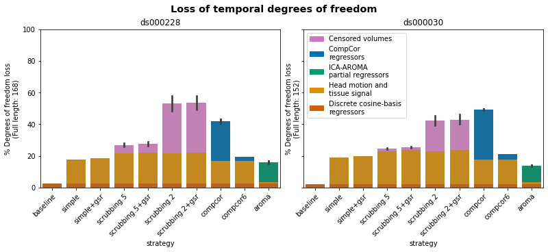
Loss of temporal degrees of freedom#
As any denoising strategy aims at a particular trade-off between the amount of noise removed and the preservation of degrees of freedom for signals, first and foremost, we would like to presentthe loss of temporal degrees of freedom.
This is an important consideration accompanying the remaining metrics.
from fmriprep_denoise.visualization import degrees_of_freedom_loss


def notebook_plot_loss_degrees_of_freedom(criteria_name, fmriprep_version):
    data = degrees_of_freedom_loss.load_data(
        path_root, datasets, criteria_name, fmriprep_version
    )
    degrees_of_freedom_loss.plot_stats(data)


criteria_name = widgets.Dropdown(
    options=["stringent", "minimal", None],
    value="stringent",
    description="Threshould: ",
    disabled=False,
)

fmriprep_version = widgets.Dropdown(
    options=["fmriprep-20.2.1lts", "fmriprep-20.2.5lts"],
    value="fmriprep-20.2.1lts",
    description="Preporcessing version : ",
    disabled=False,
)

interactive(
    notebook_plot_loss_degrees_of_freedom,
    criteria_name=criteria_name,
    fmriprep_version=fmriprep_version,
)
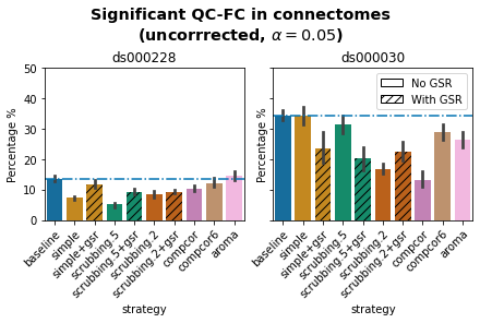
Quality control / functional connectivity (QC-FC)#
QC-FC [Power et al., 2015] quantifies the correlation between mean framewise displacement and functional connectivity. This is calculated by a partial correlation between mean framewise displacement and connectivity, with age and sex as covariates. The denoising methods should aim to reduce the QC-FC value. Significance tests associated with the partial correlations were performed, and correlations with P-values above the threshold of = 0.05 deemed significant.
from fmriprep_denoise.visualization import motion_metrics


def notebook_plot_qcfc(criteria_name, fmriprep_version):
    data, measure = motion_metrics.load_data(
        path_root, datasets, criteria_name, fmriprep_version, "p_values"
    )
    motion_metrics.plot_stats(data, measure)


fmriprep_version = widgets.Dropdown(
    options=["fmriprep-20.2.1lts", "fmriprep-20.2.5lts"],
    value="fmriprep-20.2.1lts",
    description="Preporcessing version : ",
    disabled=False,
)

interactive(
    notebook_plot_qcfc, criteria_name="stringent", fmriprep_version=fmriprep_version
)
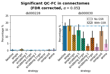
False discovery rate corrected QC-FC#
A version of this analysis corrected for multiple comparisons using the false discovery rate (Benjamini & Hochberg, 1995) is available here.
from fmriprep_denoise.visualization import motion_metrics


def notebook_plot_qcfc_fdr(criteria_name, fmriprep_version):
    data, measure = motion_metrics.load_data(
        path_root, datasets, criteria_name, fmriprep_version, "fdr_p_values"
    )
    motion_metrics.plot_stats(data, measure)


fmriprep_version = widgets.Dropdown(
    options=["fmriprep-20.2.1lts", "fmriprep-20.2.5lts"],
    value="fmriprep-20.2.1lts",
    description="Preporcessing version : ",
    disabled=False,
)

interactive(
    notebook_plot_qcfc_fdr, criteria_name="stringent", fmriprep_version=fmriprep_version
)
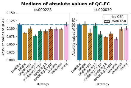
Medians of absolute values of QC-FC#
from fmriprep_denoise.visualization import motion_metrics


def notebook_plot_qcfc_median(criteria_name, fmriprep_version):
    data, measure = motion_metrics.load_data(
        path_root, datasets, criteria_name, fmriprep_version, "median"
    )
    motion_metrics.plot_stats(data, measure)


fmriprep_version = widgets.Dropdown(
    options=["fmriprep-20.2.1lts", "fmriprep-20.2.5lts"],
    value="fmriprep-20.2.1lts",
    description="Preporcessing version : ",
    disabled=False,
)

interactive(
    notebook_plot_qcfc_median,
    criteria_name="stringent",
    fmriprep_version=fmriprep_version,
)
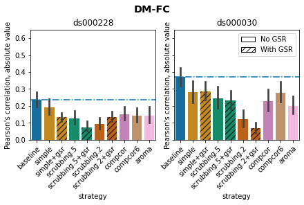
Residual distance-dependent effects of subject motion on functional connectivity (DM-FC)#
To determine the residual distance-dependence of subject movement, we first calculated the Euclidean distance between the centers of mass of each pair of parcels [Power et al., 2012]. Closer parcels generally exhibit greater impact of motion on connectivity. We then correlated the distance separating each pair of parcels and the associated QC-FC correlation of the edge connecting those parcels. We report the absolute correlation values and expect to see a general trend toward zero correlation after confound regression.
from fmriprep_denoise.visualization import motion_metrics


def notebook_plot_distance(criteria_name, fmriprep_version):
    data, measure = motion_metrics.load_data(
        path_root, datasets, criteria_name, fmriprep_version, "distance"
    )
    motion_metrics.plot_stats(data, measure)


fmriprep_version = widgets.Dropdown(
    options=["fmriprep-20.2.1lts", "fmriprep-20.2.5lts"],
    value="fmriprep-20.2.1lts",
    description="Preporcessing version : ",
    disabled=False,
)

interactive(
    notebook_plot_distance, criteria_name="stringent", fmriprep_version=fmriprep_version
)
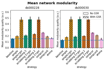
Louvain network modularity#
Confound regressors have the potential to remove real signals in addition to motion-related noise. In order to evaluate this possibility, we computed modularity quality, an explicit quantification of the degree to which there are structured subnetworks in a given network - in this case the denoised connectome [Satterthwaite et al., 2012]. Modularity quality is quantified by graph community detection based on the Louvain method [Rubinov and Sporns, 2010], implemented in the Brain Connectivity Toolbox [Rubinov and Sporns, 2010].
from fmriprep_denoise.visualization import motion_metrics


def notebook_plot_modularity(criteria_name, fmriprep_version):
    data, measure = motion_metrics.load_data(
        path_root, datasets, criteria_name, fmriprep_version, "modularity"
    )
    motion_metrics.plot_stats(data, measure)


fmriprep_version = widgets.Dropdown(
    options=["fmriprep-20.2.1lts", "fmriprep-20.2.5lts"],
    value="fmriprep-20.2.1lts",
    description="Preporcessing version : ",
    disabled=False,
)

interactive(
    notebook_plot_modularity,
    criteria_name="stringent",
    fmriprep_version=fmriprep_version,
)
Average Pearson’s correlation between mean framewise displacement and Louvain network modularity after denoising#
If confound regression and censoring were removing real signals in addition to motion-related noise, we would expect modularity to decline. To understand the extent of correlation between modularity and motion, we computed the partial correlation between subjects’ modularity values and mean framewise displacement, with age and sex as covariates.
from fmriprep_denoise.visualization import motion_metrics


def notebook_plot_modularity_motion(criteria_name, fmriprep_version):
    data, measure = motion_metrics.load_data(
        path_root, datasets, criteria_name, fmriprep_version, "modularity_motion"
    )
    motion_metrics.plot_stats(data, measure)


fmriprep_version = widgets.Dropdown(
    options=["fmriprep-20.2.1lts", "fmriprep-20.2.5lts"],
    value="fmriprep-20.2.1lts",
    description="Preporcessing version : ",
    disabled=False,
)

interactive(
    notebook_plot_modularity_motion,
    criteria_name="stringent",
    fmriprep_version=fmriprep_version,
)
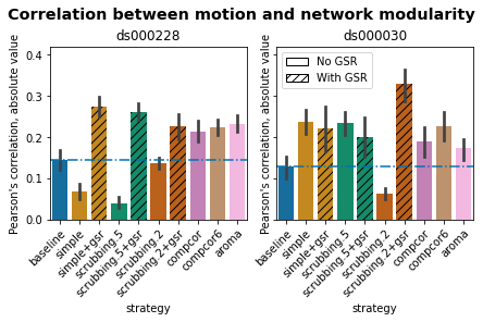
Correlation between mean framewise displacement and Louvain network modularity after denoising.#
In both datasets, the data-driven strategies and strategies with GSR performed consistently worse than baseline. The overall trend across strategies is similar to QC-FC with the exception of the baseline strategy. The reason behind this observation could be a reduction of variance in the Louvain network modularity metric for GSR-based denoising strategies.
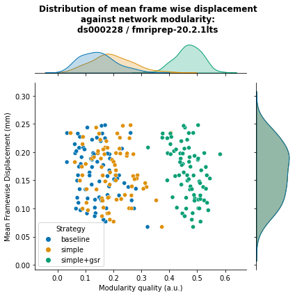
Hence, we plotted the correlations of baseline, a base strategy, a GSR variation from one parcellation scheme (DiFuMo 64 components)to demonstrate this lack of variance.
from fmriprep_denoise.visualization import motion_metrics


def notebook_plot_joint_scatter(dataset, base_strategy, fmriprep_version):
    motion_metrics.plot_joint_scatter(
        path_root, dataset, base_strategy, fmriprep_version
    )


dataset = widgets.Dropdown(
    options=["ds000228", "ds000030"],
    value="ds000228",
    description="Dataset: ",
    disabled=False,
)
fmriprep_version = widgets.Dropdown(
    options=["fmriprep-20.2.1lts", "fmriprep-20.2.5lts"],
    value="fmriprep-20.2.1lts",
    description="Preporcessing version : ",
    disabled=False,
)
base_strategy = widgets.Dropdown(
    options=["simple", "srubbing.5", "srubbing.2"],
    value="simple",
    description="Base denoise strategy ",
    disabled=False,
)

interactive(
    notebook_plot_joint_scatter,
    dataset=dataset,
    base_strategy=base_strategy,
    fmriprep_version=fmriprep_version,
)
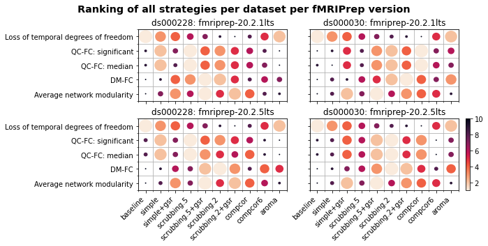
Ranking strategies from best to worst, based on four benchmark metrics#
We ranked four metrics from best to worst. Larger circles with brighter color represent higher ranking. Metric “correlation between network modularity and motion” has been excluded from the summary as it is potentially a poor measure. Loss of temporal degrees of freedom is a crucial measure that should be taken into account alongside the metric rankings.
from fmriprep_denoise.visualization import strategy_ranking


data = strategy_ranking.load_data(path_root, datasets)
fig = strategy_ranking.plot_ranking(data)