Results - Accurate Unsupervised Photon Counting from Transition Edge Sensor Signals

Results

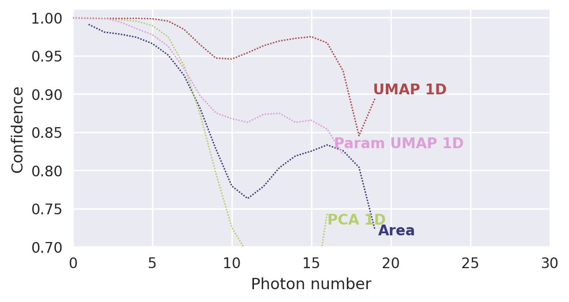
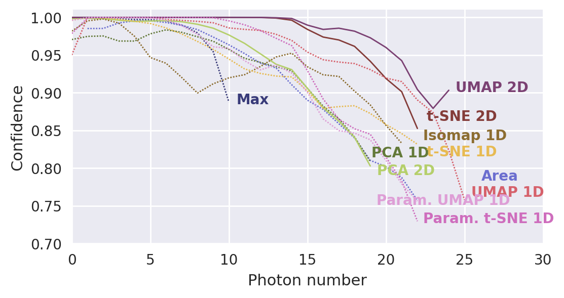
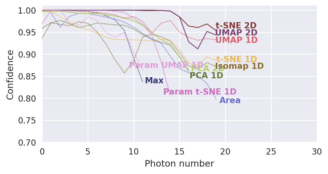
We present the confidence result for the different datasets and considering a variety of dimensionality reduction techniques.

from src.Utils import plot_results

1Synthetic Uniform¶

config_uniform = {
'MAX.npy' : {'Name' : 'Max', 'color' : '#6D7680', 'line' : (0, (1, 1)), 'n_photons' : [0,11]},
'AREA.npy' : {'Name' : 'Area', 'color' : '#6D7680', 'line' : (0, (1, 1)), 'n_photons' : [1,22]},
'PCA 1D.npy' : {'Name' : 'PCA 1D', 'color' : '#6D7680', 'line' : (0, (1, 1)), 'n_photons' : [0,20]},
'PCA 2D.npy' : {'Name' : 'PCA 2D', 'color' : '#6D7680', 'line' : '-', 'n_photons' : [0,20]},
'ISO 1D.npy' : {'Name' : 'Isomap 1D', 'color' : '#6D7680', 'line' : (0, (1, 1)), 'n_photons' : [0,22]},
'tSNE 1D.npy' : {'Name' : 't-SNE 1D', 'color' : '#E0607E', 'line' : (0, (1, 1)), 'n_photons' : [0,23]},
'tSNE 2D.npy' : {'Name' : 't-SNE 2D', 'color' : '#E0607E', 'line' : '-',  'n_photons' : [0,23]},
'UMAP 1D.npy' : {'Name' : 'UMAP 1D', 'color' : '#6D7680', 'line' : (0, (1, 1)),  'n_photons' : [0,26]},
'UMAP 2D.npy' : {'Name' : 'UMAP 2D', 'color' : '#6D7680', 'line' : '-',  'n_photons' : [0,25]},
'PTSNE 1D.npy' : {'Name' : 'Param. t-SNE 1D', 'color' : '#79AEA3', 'line' : (0, (1, 1)), 'n_photons' : [0,23]},
'PUMAP 1D.npy' : {'Name' : 'Param. UMAP 1D', 'color' : '#79AEA3', 'line' : (0, (1, 1)), 'n_photons' : [0,23]},
}

plot_results(
   config = config_uniform,
   pad = 0.5,
   xlim = (0,30),
   ylim = (0.7,1.01),
   yscale = 'linear',
   path_results = r'Results/Uniform/',
   path_results_precomp = r'Preprocess/Uniform/'
)

2Synthetic Geometric¶



config_geometric = {
'MAX.npy' : {'Name' : 'Max', 'color' : '#6D7680', 'line' : (0, (1, 1)), 'n_photons' : [0,12]},
'AREA.npy' : {'Name' : 'Area', 'color' : '#6D7680', 'line' : (0, (1, 1)), 'n_photons' : [1,19]},
'PCA 1D.npy' : {'Name' : 'PCA 1D', 'color' : '#6D7680', 'line' : (0, (1, 1)), 'n_photons' : [0,17]},
'PCA 2D.npy' : {'Name' : 'PCA 2D', 'color' : '#6D7680', 'line' : '-', 'n_photons' : [0,17]},
'ISO 1D.npy' : {'Name' : 'Isomap 1D', 'color' : '#6D7680', 'line' : (0, (1, 1)), 'n_photons' : [0,20]},
'tSNE 1D.npy' : {'Name' : 't-SNE 1D', 'color' : '#E0607E', 'line' : (0, (1, 1)), 'n_photons' : [0,20]},
'tSNE 2D.npy' : {'Name' : 't-SNE 2D', 'color' : '#E0607E', 'line' : '-',  'n_photons' : [0,20]},
'UMAP 1D.npy' : {'Name' : 'UMAP 1D', 'color' : '#6D7680', 'line' : (0, (1, 1)),  'n_photons' : [0,20]},
'UMAP 2D.npy' : {'Name' : 'UMAP 2D', 'color' : '#6D7680', 'line' : '-',  'n_photons' : [0,20]},
'PTSNE 1D.npy' : {'Name' : 'Param t-SNE 1D', 'color' : '#79AEA3', 'line' : (0, (1, 1)), 'n_photons' : [0,15]},
'PUMAP 1D.npy' : {'Name' : 'Param UMAP 1D', 'color' : '#79AEA3', 'line' : (0, (1, 1)), 'n_photons' : [0,12]},
}

plot_results(
   config = config_geometric,
   pad = 0.5,
   xlim = (0,30),
   ylim = (0.7,1.01),
   yscale = 'linear',
   path_results = r'Results/Geometric/',
   path_results_precomp = r'Preprocess/Geometric/'
)

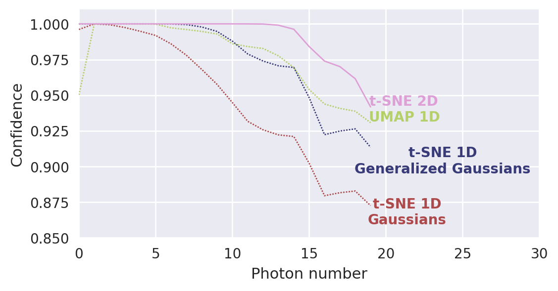
3Effect of Gaussian Mixture¶

Considering the embedding created by t-SNE is better modelled by a generalized gaussian function. To demonstrate the impact of the clustering function, we present the confidence for t-SNE modelled using a gaussian vs generalised gaussian model.

config_uniform_gauss = {
'tSNE 1D genGauss.npy' : {'Name' : 't-SNE 1D\nGeneralized Gaussians', 'color' : '#E0607E', 'line' : (0, (1, 1)), 'n_photons' : [0,20]},
'UMAP 1D.npy' : {'Name' : 'UMAP 1D', 'color' : '#6D7680', 'line' : (0, (1, 1)),  'n_photons' : [0,20]},
'tSNE 1D.npy' : {'Name' : 't-SNE 1D\nGaussians', 'color' : '#E0607E', 'line' : (0, (1, 1)), 'n_photons' : [0,20]},
'tSNE 2D.npy' : {'Name' : 't-SNE 2D', 'color' : '#E0607E', 'line' : '-',  'n_photons' : [0,20]},
}

plot_results(
   config = config_uniform_gauss,
   pad = 0.5,
   xlim = (0,30),
   ylim = (0.85,1.01),
   yscale = 'linear',
   path_results = r'Results/Uniform/',
   path_results_precomp = r'Preprocess/Uniform/'
)

4Synthetic Large¶

config_large = {
'AREA.npy' : {'Name' : 'Area', 'color' : '#6D7680', 'line' : (0, (1, 1)), 'n_photons' : [1,19]},
'PCA 1D.npy' : {'Name' : 'PCA 1D', 'color' : '#6D7680', 'line' : (0, (1, 1)), 'n_photons' : [0,17]},
'UMAP 1D.npy' : {'Name' : 'UMAP 1D', 'color' : '#6D7680', 'line' : (0, (1, 1)),  'n_photons' : [0,20]},
'PUMAP 1D.npy' : {'Name' : 'Param UMAP 1D', 'color' : '#79AEA3', 'line' : (0, (1, 1)), 'n_photons' : [0,18]},
}

plot_results(
   config = config_large,
   pad = 0.5,
   xlim = (0,30),
   ylim = (0.7,1.01),
   yscale = 'linear',
   path_results = r'Results/Large/',
   path_results_precomp = r'Preprocess/Large/'
)